
As the title suggests I’m not an expert in time series analysis, but I was curious about something and thought that some simple model could partially answer my questions. The curiosity I had in mind is to understand when there will be 100K eliminated russian occupants based on the daily losses of russian army data provided by the General Staff of Ukraine.
Below is the code and some comments to get that answer. The entire notebook and the dataset for November 6th, 2022 can be found on my GitHub. (And if you want to better understand the code I would recommend going directly there).
Data collection
To collect the data I went through all the publications by the General Staff and manually put that numbers into a Google Sheets document (it also contains the other categories of losses like tanks, vehicles, jets etc.)
Down to the business
We start with the necessary imports and initial setup which includes getting today’s data, defining the period for predictions, and defining the split date to divide the dataset into train and test to find the best fitting model.
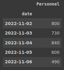
Now that we have our globals set up we can get a glimpse of the data we will be working with. It is just a two-column table with dates and losses of russians for that day. Let’s make a date column an index to ease the work with the data. We are running the .tail() command just to see if we have the most recent data.
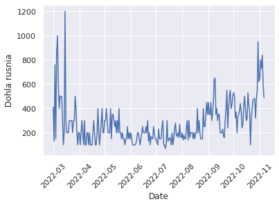
And now we can take a look at our time series on a plot
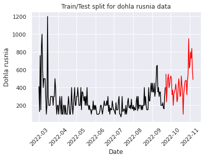
Next, we split data into train and test datasets to build a model, fit it and test it on the data we already have.
ARMA model
First I decided to go with the basic ARMA model just to get a feeling of what’s going on here and how this thing behaves.
“In the statistical analysis of time series, autoregressive–moving-average (ARMA) models provide a parsimonious description of a (weakly) stationary stochastic process in terms of two polynomials, one for the autoregression (AR) and the second for the moving average (MA). The general ARMA model was described in the 1951 thesis of Peter Whittle, Hypothesis testing in time series analysis, and it was popularized in the 1970 book by George E. P. Box and Gwilym Jenkins.” – Wikipedia.
What I have understood – it’s the basic model that might get the work done with little to no effort. So I tried:
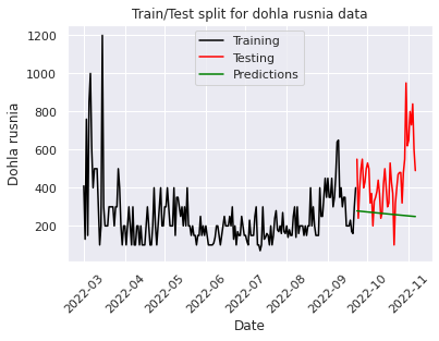
As you can see from the plot, the ARMA model with order parameters (1,0,1) draws a line that kinda makes sense, but I wanted the curve to repeat the past pattern so I went for the ARIMA model (later on I tried the best-found parameters from ARIMA for ARMA and it performed quite well).
Why the parameters 1,0,1?
“The AutoRegressive Moving Average ARMA(p,q) combines both AR(p) and MA(q) processes, considering the lagged or past values and the error terms of the time series. It is the most efficient linear model of stationary time series” – from a Medium post I used while working on this. I will list it additionally in the references.
I know, it became even more confusing. What are those parameters? – you will ask.
“The parameters of the ARIMA model are defined as follows:
- p: The number of lag observations included in the model, also called the lag order.
- d: The number of times that the raw observations are differenced, also called the degree of differencing.
- q: The size of the moving average window, also called the order of moving average.” – that’s from the fabulous blog “MachineLearningMastery”
So, as we don’t need the d parameter for the ARMA model we left it as 0.
The RMSE is also quite big – 254.4, but hey, you have the code now to play around with all these things.
ARIMA model
The next step was to play around with the ARIMA model. I will cut to the chase here: I have played around with it manually for a few hours trying to get it to work, then trying to find the best parameters of the model and later to make it a bit universal and automatic. So here is the final result.
The function evaluate_arima_model gets the data, makes a train/test split, builds a model based on the order supplied by the function params, fits it, runs a prediction on the test data, and calculates an error.
The function evaluate_model takes the dataset, a set of p, d, q values, and brute-forces the model by trying all the combinations you give it.
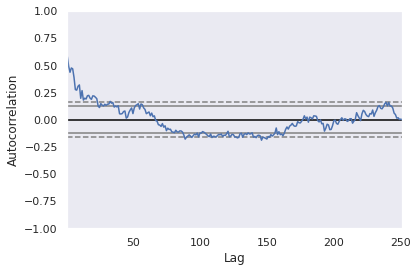
Before setting up the ranges for p, d, q values I found that you can run an autocorrelation plot on your data so it will give you a better starting point for the lag param (p). Basically, the plot says that the values above the dashed line are statistically significant lags. In this case, I would say that 20 is a good starting point, but I decided to go conservative and selected 10 as my minimum lag value.
Next thing you know you are brute-forcing all the available combinations of the parameters.
The best order found was (19, 1, 19) so I used it to fit the model on the training data again and check what the plot looks like:
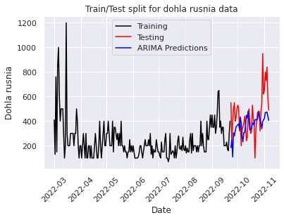
Error-values look much better here. And the predicted values more or less keep up with the real ones. RMSE = 183.07.
Once I have found the parameters that work best for the given dataset I decided to make the predictions for the next 45 days using all the data. Below is the code for that.
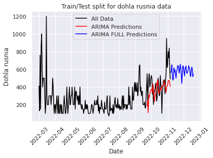
And a quick loop to find out the day of 100K

That’s it, 4 days of data collection, learning, investigation, and parameter tuning and here you have an article with basics on how to perform time series analysis for the dummies from a dummy. I think this is a good starting point and definitely there is a lot that can be improved here. As I lack knowledge in this domain I just don’t know what that can be 😀
Also, I will be running this model on my machine every day just to see how it behaves with time passing by and new data points. Because what I have noticed is that the model depends a lot on the last data point so it will be interesting to see how it changes with time. Another good idea might be to perform hyperparameter tuning every once in a while to see if I can get better results.
I hope you learned something while reading this! See you in the next one 🙂
Sources:
- Autoregressive–moving-average model
- How to Create an ARIMA Model for Time Series Forecasting in Python – Machine Learning Mastery
- Identifying the numbers of AR or MA terms in an ARIMA model
- Find the order of ARIMA models
- How to Grid Search ARIMA Model Hyperparameters with Python – Machine Learning Mastery
Photo by Josh Rakower on Unsplash